A First Look at Self-Attention#
Consider the following review:
“The movie was not good, but the soundtrack was amazing.”
A simple bag-of-words classifier will see both good and amazing (positive) and probably predict a positive sentiment, missing the negation “not.”
Self-attention can discover that “not” modifies “good” while leaving “amazing” untouched.
The first step is to tokenize the sentence:
position |
token |
|---|---|
0 |
The |
1 |
movie |
2 |
was |
3 |
not |
4 |
good |
5 |
, |
6 |
but |
7 |
the |
8 |
soundtrack |
9 |
was |
10 |
amazing |
11 |
. |
Each token is mapped to a small vector (embedding). The exact numbers are not important; they are learned during training. In fact, a positional embedding is used to also indicate its position in the sentence.
Computing attention scores (conceptually)#
Focus on the token at position 4, “good.” We want to compute how much attention it should pay to all other tokens in the sentence. To find this, we do the following:
Query and key vectors: For each token, we compute three vectors: a query \(q_i\) and a key \(k_j\). These are obtained by multiplying the embedding with learned weight matrices \(W^Q\) and \(W^K\). The value vector \(v_j\) is also computed, but it is not used to compute the attention scores.
Dot product: For the token at position 4, we compute the dot product of its query \(q_{good}\) with all keys \(k_j\) in the sentence. This gives us a score for each token, indicating how relevant it is to the token at position 4. Larger dot products mean higher relevance. Then, after scaling and the applying softmax, we obtain a weight for each other token:
key token \(j\)
weight \(w_{4j}\)
The
0.01
movie
0.02
was (1st)
0.03
not
0.55
good
0.10
,
0.02
but
0.05
the
0.02
soundtrack
0.03
was (2nd)
0.05
amazing
0.11
.
0.01
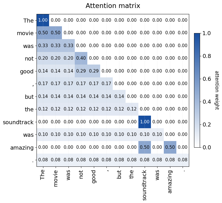
In this example, the model assigns more than half of the total weight to “not,” capturing the local negation, and a moderate share to “amazing,” which influences the overall sentiment.
Weighted sum of value vectors: In addition to query and key vectors, we also compute a value vector \(v_j\). Finally, we compute a weighted sum of the value vectors \(v_j\) using the weights \(w_{4j}\): $\( \text{output}(\text{good}) =\sum_{j=0}^{11} w_{4j}\,v_j . \)$
Because \(w_{4,3}=0.55\) is large, the output vector encodes that “good” is negated.
Later layers (or a classifier head) can use this context-rich vector to predict a negative contribution from “not good,” while recognising the strong positive signal from “amazing.”
Summary#
Context matters. Self-attention lets every token look at the entire sentence, so “not” can influence “good.”
Parallel computation. Unlike an RNN, all tokens are processed at once, which is faster and handles long sentences gracefully.
Dynamic meaning. The same word can mean something different in another sentence; the attention pattern adapts.
Quick refresher on the dot product#
For two vectors \(\mathbf a, \mathbf b \in \mathbb R^{d}\) with
\(\mathbf a = (a_1,\dots,a_d)\) and \(\mathbf b = (b_1,\dots,b_d)\), the the dot product is defined as:
For example, consider the two vectors:
a = [2, 3]
b = [5, −1]
To find the dot product, we multiply the corresponding elements and sum them up:
a · b = 2·5 + 3·(−1) = 10 − 3 = 7
Geometric view#
where \(\theta\) is the angle between the vectors.
angle \(\theta\) |
\(\cos\theta\) |
sign / size of \(\mathbf a\!\cdot\!\mathbf b\) |
geometric relation |
|---|---|---|---|
\(0^\circ\) |
\(+1\) |
largest positive |
vectors point the same way |
\(90^\circ\) |
\(0\) |
zero |
vectors are orthogonal |
\(180^\circ\) |
\(-1\) |
negative |
vectors point opposite ways |
A high positive dot product implies that vectors are long and almost parallel. A zero dot product implies that the vectors are orthogonal (perpendicular). A negative dot product implies that the vectors are long and almost opposite.
Why dot products drive self-attention#
Query \(q_i\) = direction token i is “looking”
Key \(k_j\) = direction of token j’s features
Score \(s_{i,j}=q_i\!\cdot k_j\)
Large \(s_{i,j}\) implies a small angle between the vectors which implies that token j matches what token i wants.
import numpy as np

q_good = np.array([0, 1])      # query for "good"
k_good = np.array([0, 1])      # key   for "good"
k_not  = np.array([0.5, 0.5])  # key   for "not"
k_the  = np.array([0,  0])     # key   for "The"

scores = np.array([
    q_good @ k_good,   # 1.0
    q_good @ k_not,    # 0.5
    q_good @ k_the     # 0.0
])

scores /= np.sqrt(2)
weights = np.exp(scores) / np.exp(scores).sum()

print("Weights from 'good' → good, not, The")
print(np.round(weights, 2))
Weights from 'good' → good, not, The
[0.46 0.32 0.22]
Query Q, Key K, and Value V Matrices#
Suppose that \(n\) is the sequence length, \(d_{\text{model}}\) is the embedding dimension, and \(d_k\) is the dimension of the query, key and value vectors.
\(n\) is the number of tokens in the input sequence after truncation and padding.
\(d_{\text{model}}\) is the size of the embedding vector for each token.
\(d_k\) is the size of the query, key, and value vectors. The model keeps three learned weight matrices \(W_Q\), \(W_K\), and \(W_V\) of size \(d_{\text{model}} \times d_k\).
Let \(X \in \mathbb{R}^{n \times d_{\text{model}}}\) be the matrix whose rows are the token-embedding vectors after positional encoding
For each attention head \(h\) the model keeps three learned weight matrices
Multiplying the embedding matrix by those weights yields
The shape of each of \(Q, K, V\) is \(n \times d_k\) (one \(d_k\)-dimensional row per token). The rows \(q_i,\;k_i,\;v_i\) are the query, key, and value vectors for token \(i\).
Symbol |
Intuitive meaning |
|---|---|
\(q_i\) |
“What does this token need or look for?” |
\(k_j\) |
“What attributes does token j offer to others?” |
\(v_j\) |
“The information token j will contribute if it is attended to.” |
import numpy as np

# ---------------------------------------------------------------------
# 1) Token list – indices are handy for debugging
# ---------------------------------------------------------------------
tokens = ["The", "movie", "was", "not", "good", ",", "but",
          "the", "soundtrack", "was", "amazing", "."]

n_tokens, d = len(tokens), 2                # d_model = 2
Q = np.zeros((n_tokens, d))
K = np.zeros((n_tokens, d))
V = np.zeros((n_tokens, d))

# ---------------------------------------------------------------------
# 2) Hand-crafted vectors for the three special words
# ---------------------------------------------------------------------
special_qk = {3: [20, 20],      # “not”
              4: [0, 1],      # “good”
             10: [19, 19]}      # “amazing”

special_v  = {3: [1, 0],
              4: [0, 1],
             10: [1, 1]}

for idx, vec in special_qk.items():
    Q[idx] = K[idx] = vec

for idx, vec in special_v.items():
    V[idx] = vec

# ---------------------------------------------------------------------
# 3) Scaled dot-product attention  (decoder style → add causal mask)
# ---------------------------------------------------------------------
scores = Q @ K.T                           # (n_tokens × n_tokens)
scores /= np.sqrt(d)                       # scale by √d_k

# ---- causal (look-ahead) mask ----
#mask = np.triu(np.ones_like(scores, dtype=bool), k=1)  # j > i region
#scores[mask] = -1e9                      # −∞ ⇒ 0 after softmax

# Softmax row by row
exp_scores = np.exp(scores)
weights = exp_scores / exp_scores.sum(axis=-1, keepdims=True)

# ---------------------------------------------------------------------
# 4) Attention output = weights · V
# ---------------------------------------------------------------------
outputs = weights @ V                      # (n_tokens × d)

# ---------------------------------------------------------------------
# 5) Inspect the row that corresponds to the *query* word “good”
# ---------------------------------------------------------------------
idx_good = 4
print(f"\nMasked attention weights FROM ‘{tokens[idx_good]}’ (index {idx_good})")
for j, w in enumerate(weights[idx_good]):
    print(f"  → {tokens[j]:<11s}  w = {w:.2f}")

print("\nResulting context vector for 'good':", outputs[idx_good])
Masked attention weights FROM ‘good’ (index 4)
  → The          w = 0.00
  → movie        w = 0.00
  → was          w = 0.00
  → not          w = 0.67
  → good         w = 0.00
  → ,            w = 0.00
  → but          w = 0.00
  → the          w = 0.00
  → soundtrack   w = 0.00
  → was          w = 0.00
  → amazing      w = 0.33
  → .            w = 0.00

Resulting context vector for 'good': [0.99999467 0.33023767]
import numpy as np
import matplotlib.pyplot as plt
from matplotlib.colors import LinearSegmentedColormap

# --------------------------------------------------------------------
# 1) Sentence tokens and tiny hand-crafted projections
# --------------------------------------------------------------------
tokens = [
    "The", "movie", "was", "not", "good", ",", "but",
    "the", "soundtrack", "was", "amazing", "."
]
n, d = len(tokens), 2           # d_model = d_k = 2  (tiny for clarity)

# Hand-crafted query/key vectors for three important words
special_qk = {
     3: [0, 1],   # "not"
     4: [ 0,  1],   # "good"
    8: [19, 19],   # "soundtrack"
    10: [19, 19]    # "amazing"
}

# Hand-crafted value vectors (not used for the heat-map itself)
special_v = {
     3: [-1, 0], # not
     4: [0, 1],  # good
    8: [1, 1],   # amazing
    10: [1, 1]   # amazing
}

# --------------------------------------------------------------------
# 2) Build Q, K and compute the masked attention weights
# --------------------------------------------------------------------
def build_QK():
    Q = np.zeros((n, d))
    K = np.zeros((n, d))
    for idx, vec in special_qk.items():
        Q[idx] = K[idx] = vec
    return Q, K

def attention_with_causal_mask():
    Q, K = build_QK()
    scores = (Q @ K.T) / np.sqrt(d)                # scaled dot products
    # causal mask = forbid future tokens (j > i)
    future = np.triu(np.ones_like(scores, dtype=bool), k=1)
    scores[future] = -1e9                          # -∞ so softmax → 0
    exp_s = np.exp(scores)
    W = exp_s / exp_s.sum(axis=-1, keepdims=True)  # row-softmax
    return W

W_mask = attention_with_causal_mask()

# --------------------------------------------------------------------
# 3) Figure aesthetics (bigger fonts, custom white→blue colormap)
# --------------------------------------------------------------------
plt.rcParams.update({"font.size": 14})

white_blue = LinearSegmentedColormap.from_list(
    "white_blue", ["#ffffff", "#184fa0"]
)

fig = plt.figure(figsize=(8, 8))
ax = fig.add_subplot(111)

im = ax.imshow(W_mask, cmap=white_blue, vmin=0, vmax=W_mask.max())

# axis ticks and labels
ax.set_xticks(range(n))
ax.set_yticks(range(n))
ax.set_xticklabels(tokens, rotation=90)
ax.set_yticklabels(tokens)
ax.set_title("Attention matrix", pad=15)

# numeric annotations (show every cell, even zeros)
for i in range(n):
    for j in range(n):
        val = W_mask[i, j]
        text_color = "white" if val > 0.6 * W_mask.max() else "black"
        ax.text(j, i, f"{val:.2f}", ha="center", va="center",
                color=text_color, fontsize=11)

# colour-bar
cbar = fig.colorbar(im, fraction=0.035, pad=0.03)
cbar.set_label("attention weight", rotation=270, labelpad=20, fontsize=12)

# light grid for readability
ax.grid(which="both", color="lightgray", linewidth=0.25, linestyle="--", zorder=-1)

plt.tight_layout()
plt.show()
Example: Self-attention in action#
The following code builds the smallest possible Transformer-style model to show how self-attention works on synthetic data.
Each sample is a seven-token sentence that begins with a special classification token [CLS] = 0, followed by six random integers 1 – 50.
The binary label is 1 when the fourth random token (position 4) equals 42, and 0 otherwise.
The model consists of the following components:
Embeddings – A learnable token embedding and a learnable positional embedding of dimension 8 are summed to give a \(\text{seq\_len}\times d_{\text{model}}\) input matrix.
Single-head self-attention – Queries, keys, and values are all the same embedded sequence, so the layer learns how much each position attends to every other position.
Read-out via [CLS] – After attention the updated vector at position 0 ([CLS]) is taken as a fixed-length representation of the whole sentence; a single sigmoid unit turns it into the predicted probability.
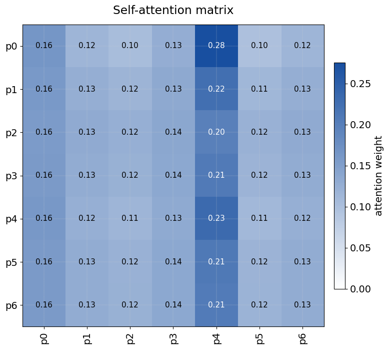
This code demonstrates how a Transformer can learn to focus nearly all its attention on the task-relevant token (position 4) and route that information through the [CLS] vector to make a classification decision.
# ------------------------------------------------------------- #
#  Tiny self-attention demo                                     #
# ------------------------------------------------------------- #
import tensorflow as tf
from tensorflow.keras import layers, Model
import numpy as np
import matplotlib.pyplot as plt
from matplotlib.colors import LinearSegmentedColormap

# 0) Reproducibility
tf.random.set_seed(0)
np.random.seed(0)

# 1) Synthetic data  (create fresh every run)
VOCAB_SIZE  = 51        # integers 1‒50, plus 0 for [CLS]
BASE_LEN    = 6         # six random tokens
NUM_SAMPLES = 8_000
EPOCHS      = 10

rand_tokens = np.random.randint(1, VOCAB_SIZE, size=(NUM_SAMPLES, BASE_LEN))
tokens_np   = np.concatenate(
                 [np.zeros((NUM_SAMPLES, 1), dtype=int),   # [CLS] = 0
                  rand_tokens],
                 axis=1)                                   # shape (N, 7)

labels_np   = (tokens_np[:, 4] == 42).astype("float32")    # is token-4 == 42?
SEQ_LEN     = tokens_np.shape[1]                          # 7

class PositionalEmbedding(layers.Layer):
    def __init__(self, vocab, d_model, max_len, **kw):
        super().__init__(**kw)
        self.tok = layers.Embedding(vocab,   d_model)
        self.pos = layers.Embedding(max_len, d_model)
    def call(self, tok_ids):
        L = tf.shape(tok_ids)[1]
        return self.tok(tok_ids) + self.pos(tf.range(L))

D_MODEL = 8
inp  = layers.Input((SEQ_LEN,), dtype="int32")
emb  = PositionalEmbedding(VOCAB_SIZE, D_MODEL, SEQ_LEN)(inp)

mha = layers.MultiHeadAttention(
        num_heads=1,
        key_dim=D_MODEL,
        output_shape=D_MODEL,
        name="self_attn")

attn_out, attn_scores = mha(
        emb,             # query
        emb,             # value  (same, so self-attention)
        return_attention_scores=True)
x        = layers.LayerNormalization(epsilon=1e-6)(emb + attn_out)
cls_vec  = x[:, 0, :]
logits   = layers.Dense(1, activation="sigmoid")(cls_vec)

model = Model(inp, logits)
model.compile(optimizer="adam", loss="binary_crossentropy", metrics=["accuracy"])

ds = (tf.data.Dataset.from_tensor_slices((tokens_np, labels_np))
        .shuffle(NUM_SAMPLES)
        .batch(32))
model.fit(ds, epochs=EPOCHS, verbose=0)

# Extract attention for the first sample
A = Model(inp, attn_scores).predict(tokens_np[:1], verbose=0)[0, 0]  # (7, 7)

# Plot heat-map
positions = [f"p{i}" for i in range(SEQ_LEN)]
plt.rcParams.update({"font.size": 14})
cmap = LinearSegmentedColormap.from_list("wb", ["#ffffff", "#184fa0"])

fig, ax = plt.subplots(figsize=(8, 8))
im = ax.imshow(A, cmap=cmap, vmin=0, vmax=A.max())

ax.set_xticks(range(SEQ_LEN)); ax.set_xticklabels(positions, rotation=90)
ax.set_yticks(range(SEQ_LEN)); ax.set_yticklabels(positions)
ax.set_title("Self-attention matrix", pad=15)

for i in range(SEQ_LEN):
    for j in range(SEQ_LEN):
        val = A[i, j]
        ax.text(j, i, f"{val:.2f}",
                ha="center", va="center",
                color="white" if val > 0.6*A.max() else "black", fontsize=11)

fig.colorbar(im, fraction=0.035, pad=0.03,
             label="attention weight")
ax.grid(which="both", color="lightgray", linewidth=0.25, linestyle="--", zorder=-1)
plt.tight_layout()
plt.show()
print("Sentence-0:", tokens_np[0])
print("Token at pos-3:", tokens_np[0, 3])
pred = model.predict(tokens_np[:1])[0, 0]
print("Model output for sample-0:", pred)   # should be ≪ 0.5

idx = np.where(labels_np == 1)[0][0]   # first positive sample
print(f"Sentence-{idx}:", tokens_np[idx])
print(model.predict(tokens_np[idx:idx+1])[0, 0])  # should be ≫ 0.5

loss, acc = model.evaluate(ds, verbose=0)
print(f"Model accuracy: {acc:.2%}")
print(f"Model loss: {loss:.4f}")
print("Model summary:")
model.summary()
Sentence-0: [ 0 45 48  1  4  4 40]
Token at pos-3: 1
1/1 ━━━━━━━━━━━━━━━━━━━━ 0s 62ms/step
Model output for sample-0: 0.000100963625
Sentence-103: [ 0 34 13 33 42 17  3]
1/1 ━━━━━━━━━━━━━━━━━━━━ 0s 17ms/step
0.9992883
Model accuracy: 100.00%
Model loss: 0.0001
Model summary:
Model: "functional_21"
┏━━━━━━━━━━━━━━━━━━━━━┳━━━━━━━━━━━━━━━━━━━┳━━━━━━━━━━━━┳━━━━━━━━━━━━━━━━━━━┓
┃ Layer (type)        ┃ Output Shape      ┃    Param # ┃ Connected to      ┃
┡━━━━━━━━━━━━━━━━━━━━━╇━━━━━━━━━━━━━━━━━━━╇━━━━━━━━━━━━╇━━━━━━━━━━━━━━━━━━━┩
│ input_layer_10      │ (None, 7)         │          0 │ -                 │
│ (InputLayer)        │                   │            │                   │
├─────────────────────┼───────────────────┼────────────┼───────────────────┤
│ positional_embeddi… │ (None, 7, 8)      │        464 │ input_layer_10[0… │
│ (PositionalEmbeddi… │                   │            │                   │
├─────────────────────┼───────────────────┼────────────┼───────────────────┤
│ self_attn           │ [(None, 7, 8),    │        288 │ positional_embed… │
│ (MultiHeadAttentio… │ (None, 1, 7, 7)]  │            │ positional_embed… │
├─────────────────────┼───────────────────┼────────────┼───────────────────┤
│ add_26 (Add)        │ (None, 7, 8)      │          0 │ positional_embed… │
│                     │                   │            │ self_attn[0][0]   │
├─────────────────────┼───────────────────┼────────────┼───────────────────┤
│ layer_normalizatio… │ (None, 7, 8)      │         16 │ add_26[0][0]      │
│ (LayerNormalizatio… │                   │            │                   │
├─────────────────────┼───────────────────┼────────────┼───────────────────┤
│ get_item_22         │ (None, 8)         │          0 │ layer_normalizat… │
│ (GetItem)           │                   │            │                   │
├─────────────────────┼───────────────────┼────────────┼───────────────────┤
│ dense_10 (Dense)    │ (None, 1)         │          9 │ get_item_22[0][0] │
└─────────────────────┴───────────────────┴────────────┴───────────────────┘
Total params: 2,333 (9.12 KB)
Trainable params: 777 (3.04 KB)
Non-trainable params: 0 (0.00 B)
Optimizer params: 1,556 (6.08 KB)