Convnets - Convolutional Neural Networks

Convolutional Neural Networks (CNNs) are a class of deep learning models specifically designed for processing structured grid data, such as images. They are particularly effective for tasks like image classification, object detection, and segmentation.

We start with an example to illustrate the basic components of a CNN. The following code demonstrates a simple CNN that classifies images from the MNIST dataset of handwritten digits. The model consists of several convolutional layers followed by fully connected layers.

from tensorflow import keras 
#from tensorflow.keras import layers 

# Input layer for 28x28 grayscale images
inputs = keras.Input(shape=(28, 28, 1))

# Convolutional layers
x = layers.Conv2D(filters=32, kernel_size=3, activation="relu")(inputs)
x = layers.MaxPooling2D(pool_size=2)(x)
x = layers.Conv2D(filters=64, kernel_size=3, activation="relu")(x)
x = layers.MaxPooling2D(pool_size=2)(x)
x = layers.Conv2D(filters=128, kernel_size=3, activation="relu")(x)

# Flattening before Dense layers
x = layers.Flatten()(x)

# Dense (fully-connected) output layer
outputs = layers.Dense(10, activation="softmax")(x)

# Define the model
model = keras.Model(inputs=inputs, outputs=outputs)

# View the model structure clearly
model.summary()

2025-05-08 15:04:22.923822: I external/local_xla/xla/tsl/cuda/cudart_stub.cc:32] Could not find cuda drivers on your machine, GPU will not be used.
2025-05-08 15:04:22.927026: I external/local_xla/xla/tsl/cuda/cudart_stub.cc:32] Could not find cuda drivers on your machine, GPU will not be used.
2025-05-08 15:04:22.935483: E external/local_xla/xla/stream_executor/cuda/cuda_fft.cc:467] Unable to register cuFFT factory: Attempting to register factory for plugin cuFFT when one has already been registered
WARNING: All log messages before absl::InitializeLog() is called are written to STDERR
E0000 00:00:1746716662.949376   54056 cuda_dnn.cc:8579] Unable to register cuDNN factory: Attempting to register factory for plugin cuDNN when one has already been registered
E0000 00:00:1746716662.953552   54056 cuda_blas.cc:1407] Unable to register cuBLAS factory: Attempting to register factory for plugin cuBLAS when one has already been registered
W0000 00:00:1746716662.964779   54056 computation_placer.cc:177] computation placer already registered. Please check linkage and avoid linking the same target more than once.
W0000 00:00:1746716662.964789   54056 computation_placer.cc:177] computation placer already registered. Please check linkage and avoid linking the same target more than once.
W0000 00:00:1746716662.964790   54056 computation_placer.cc:177] computation placer already registered. Please check linkage and avoid linking the same target more than once.
W0000 00:00:1746716662.964792   54056 computation_placer.cc:177] computation placer already registered. Please check linkage and avoid linking the same target more than once.
2025-05-08 15:04:22.969013: I tensorflow/core/platform/cpu_feature_guard.cc:210] This TensorFlow binary is optimized to use available CPU instructions in performance-critical operations.
To enable the following instructions: AVX2 FMA, in other operations, rebuild TensorFlow with the appropriate compiler flags.

---------------------------------------------------------------------------
NameError                                 Traceback (most recent call last)
Cell In[1], line 8
      5 inputs = keras.Input(shape=(28, 28, 1))
      7 # Convolutional layers
----> 8 x = layers.Conv2D(filters=32, kernel_size=3, activation="relu")(inputs)
      9 x = layers.MaxPooling2D(pool_size=2)(x)
     10 x = layers.Conv2D(filters=64, kernel_size=3, activation="relu")(x)

NameError: name 'layers' is not defined

from tensorflow.keras.datasets import mnist

(train_images, train_labels), (test_images, test_labels) = mnist.load_data() 

train_images = train_images.reshape((60000, 28, 28, 1))
train_images = train_images.astype("float32") / 255 
test_images = test_images.reshape((10000, 28, 28, 1)) 
test_images = test_images.astype("float32") / 255

model.compile(optimizer="rmsprop",
              loss="sparse_categorical_crossentropy",
              metrics=["accuracy"])

history = model.fit(train_images, train_labels, epochs=5, batch_size=64, verbose=0)

test_loss, test_acc = model.evaluate(test_images, test_labels)

print("Test loss ", test_loss)
print("Test accuracy ", test_acc)

313/313 ━━━━━━━━━━━━━━━━━━━━ 1s 4ms/step - accuracy: 0.9897 - loss: 0.0325
Test loss  0.023203570395708084
Test accuracy  0.9930999875068665

Dense vs. Convolutional Layers

Dense (Fully-connected) Layers

• Global Patterns: Dense layers learn patterns involving all pixels at once.

• Example:
  Recognizing digits by overall patterns (e.g., “an image with two loops could be digit 8”).

Convolutional Layers

• Local Patterns: Convolutional layers learn patterns from small regions (windows) of the image, typically \(3\times 3\).

• Example:
  Detecting edges, curves, or intersections locally, like recognizing a vertical line or corner.

In the above example, we have the following layers:

Layer	Patterns learned	Example (MNIST digit recognition)
Conv2D (filters=32)	Simple local patterns (edges, lines)	Vertical edges, horizontal edges, small curves
Conv2D (filters=64)	More complex local patterns	Corners, intersections, curved shapes
Conv2D (filters=128)	Richer, detailed local patterns	Loops, combined shapes, parts of digits
Flatten	Combines local features into vector	Prepares local features for global interpretation
Dense (10 neurons)	Global patterns	Combines local features to classify digits globally

• Convolutional layers excel at extracting local, spatial features efficiently.

• Dense layers integrate these extracted features globally for effective classification.

import matplotlib.pyplot as plt
from tensorflow.keras.models import Model
from tensorflow.keras.datasets import mnist
from tensorflow.keras import layers, Input

# Load MNIST image
(train_images, _), _ = mnist.load_data()
img = train_images[1] / 255.0
img_input = img.reshape(1,28,28,1)

# Define convolutional model with 4 filters
inputs = Input(shape=(28,28,1))
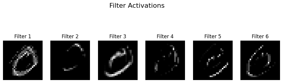
conv = layers.Conv2D(100, kernel_size=3, activation='relu')(inputs)
model = Model(inputs, conv)

# Get feature maps
feature_maps = model.predict(img_input)

# Plot feature maps
fig, axes = plt.subplots(1, 6, figsize=(12,4))
for i in range(6):
    axes[i].imshow(feature_maps[0,:,:,i], cmap='gray')
    axes[i].axis('off')
    axes[i].set_title(f'Filter {i+1}')
plt.suptitle('Filter Activations', fontsize=16)
plt.show()

1/1 ━━━━━━━━━━━━━━━━━━━━ 0s 25ms/step

Example: Convolution and the Sum of Two Dice

A fair die has 6 outcomes, each with probability \(\frac{1}{6}\):

Roll	Probability
1	\(\frac{1}{6}\)
2	\(\frac{1}{6}\)
3	\(\frac{1}{6}\)
4	\(\frac{1}{6}\)
5	\(\frac{1}{6}\)
6	\(\frac{1}{6}\)

When rolling two dice, the probability of each possible sum (from 2 to 12) is calculated using a convolution:

\[ P(X + Y = z) = \sum_k P(X = k) \cdot P(Y = z - k) \]

Sum	Combinations	Number of Ways	Probability
2	(1,1)	1	\(\frac{1}{36}\)
3	(1,2), (2,1)	2	\(\frac{2}{36}\)
4	(1,3), (2,2), (3,1)	3	\(\frac{3}{36}\)
5	(1,4), (2,3), (3,2), (4,1)	4	\(\frac{4}{36}\)
6	(1,5), (2,4), (3,3), (4,2), (5,1)	5	\(\frac{5}{36}\)
7	(1,6), (2,5), (3,4), (4,3), (5,2), (6,1)	6	\(\frac{6}{36}\)
8	(2,6), (3,5), (4,4), (5,3), (6,2)	5	\(\frac{5}{36}\)
9	(3,6), (4,5), (5,4), (6,3)	4	\(\frac{4}{36}\)
10	(4,6), (5,5), (6,4)	3	\(\frac{3}{36}\)
11	(5,6), (6,5)	2	\(\frac{2}{36}\)
12	(6,6)	1	\(\frac{1}{36}\)

Given two vectors (or sequences) \(f\) and \(g\), the convolution of \(f\) and \(g\) is a new vector defined mathematically as follows:

\[ (f * g)[n] = \sum_{k} f[k] \cdot g[n - k] \]

• \(f\) and \(g\): The two input vectors being convolved.

• \((f * g)\): The convolution of \(f\) and \(g\).

• \((f * g)[n]\): The value at position \(n\) in the resulting convolution vector.

• The summation runs over all indices \(k\) for which both \(f[k]\) and \(g[n - k]\) are defined.

If the length of \(f\) is \(m\) and the length of \(g\) is \(n\), then the convolution \((f * g)\) has length: $\( m + n - 1 \)$

Intuition: The convolution operation is like sliding one vector over another, multiplying corresponding overlapping elements, and summing the products at each step. This operation appears frequently in probability, signal processing, and neural networks.

Simple Convolution Example

Consider two short vectors:

• \(f = [1, 2, 3]\)

• \(g = [4, 5]\)

The convolution is defined as:

\[ (f * g)[n] = \sum_k f[k] \cdot g[n - k] \]

Let’s perform the convolution explicitly, step by step:

• Step 1: \((f * g)[0]\)

\[ (f * g)[0] = f[0] \cdot g[0] = (1)(4) = 4 \]

• *Step 2: \((f * g)[1]\)

\[ (f * g)[1] = f[0] \cdot g[1] + f[1] \cdot g[0] = (1)(5) + (2)(4) = 5 + 8 = 13 \]

• Step 3: \((f * g)[2]\)

\[ (f * g)[2] = f[1] \cdot g[1] + f[2] \cdot g[0] = (2)(5) + (3)(4) = 10 + 12 = 22 \]

• Step 4: \((f * g)[3]\)

\[ (f * g)[3] = f[2] \cdot g[1] = (3)(5) = 15 \]

• Final Result:

\[ f * g = [4, 13, 22, 15] \]

import numpy as np

f = np.array([1, 2, 3])
g = np.array([4, 5])
# convolution 
print(f"{f}*{g} = {np.convolve(f, g, mode='full')}")

[1 2 3]*[4 5] = [ 4 13 22 15]

# probabilities of a single fair die
die = np.array([1/6]*6)

# convolution of two dice
sum_two_dice = np.convolve(die, die, mode='full')

print(sum_two_dice)

[0.02777778 0.05555556 0.08333333 0.11111111 0.13888889 0.16666667
 0.13888889 0.11111111 0.08333333 0.05555556 0.02777778]

die = np.array([1/6]*6)
bias_coin = [0.3, 0.7]
sum_pr = np.convolve(die, bias_coin, mode='full')

print(sum_pr)

print(np.sum(sum_pr))

[0.05       0.16666667 0.16666667 0.16666667 0.16666667 0.16666667
 0.11666667]
0.9999999999999999

2D Convolution: Mathematical Definition and Simple Example

Given two 2-dimensional arrays (matrices) \(I\) (the input) and \(K\) (the kernel), their 2D convolution \((I * K)\) is defined mathematically as follows:

\[ (I * K)[x,y] = \sum_{m}\sum_{n} I[m,n] \cdot K[x - m,\, y - n] \]

• Typically, the kernel \(K\) is smaller than the input array \(I\).

• The kernel is flipped horizontally and vertically in mathematical convolution before performing multiplication and summation.

Consider the following simple example:

Input array \(I\) (3×3): $\( I = \begin{bmatrix} 1 & 2 & 1 \\ 0 & 1 & 0 \\ 2 & 1 & 3 \end{bmatrix} \)$

Kernel \(K\) (2×2): $\( K = \begin{bmatrix} 1 & 0 \\ -1 & 1 \end{bmatrix} \)$

First, remember convolution involves flipping the kernel both horizontally and vertically. Thus, the flipped kernel becomes:

\[\begin{split} K_{\text{flipped}} = \begin{bmatrix} 1 & -1 \\ 0 & 1 \end{bmatrix} \end{split}\]

We slide the flipped kernel over the input array and perform element-wise multiplication and summation at each position.

• Position (0,0) (top-left):

\[ (1)(1) + (2)(-1) + (0)(0) + (1)(1) = 1 - 2 + 0 + 1 = 0 \]

• Position (0,1) (top-middle):

\[ (2)(1) + (1)(-1) + (1)(0) + (0)(1) = 2 - 1 + 0 + 0 = 1 \]

• Position (1,0) (middle-left):

\[ (0)(1) + (1)(-1) + (2)(0) + (1)(1) = 0 - 1 + 0 + 1 = 0 \]

• Position (1,1) (middle-middle):

\[ (1)(1) + (0)(-1) + (1)(0) + (3)(1) = 1 + 0 + 0 + 3 = 4 \]

Thus, clearly, the final convolution result (valid mode) is:

\[\begin{split} I * K = \begin{bmatrix} 0 & 1 \\ 0 & 4 \end{bmatrix} \end{split}\]

• 2D Convolution: Flip kernel, slide over the input, multiply corresponding elements, sum results at each step.

• Resulting matrix dimension (no padding): $\( (\text{input size}) - (\text{kernel size}) + 1 \)$

• Each resulting number measures how strongly each region matches the kernel’s pattern.

import numpy as np
from scipy.signal import convolve2d
from scipy.signal import correlate2d
image = np.array([
 [1, 2, 1], 
 [0, 1, 0],
 [2, 1, 3]
])

kernel = np.array([
    [1, 0],
    [-1, 1]
])

# Perform 2D convolution
result = convolve2d(image, kernel, mode='valid')

print("convolution\n", result)

result = correlate2d(image, kernel, mode='valid')
print("correlate\n",result)

convolution
 [[0 1]
 [0 4]]
correlate
 [[ 2  1]
 [-1  3]]

import numpy as np
from scipy.signal import convolve2d
from scipy.signal import correlate2d


# Example 5x5 input array (image)
image = np.array([
    [1, 2, 3, 0, 1],
    [0, 1, 2, 3, 4],
    [1, 0, 1, 2, 3],
    [0, 1, 0, 1, 2],
    [3, 2, 1, 0, 1]
])

# Example 2x2 kernel
kernel = np.array([
    [1, 0],
    [-1, 1]
])

# Perform 2D convolution
result = convolve2d(image, kernel, mode='valid')

print(result)

result = correlate2d(image, kernel, mode='valid')
print(result)

[[ 0  1  6  3]
 [-1  0  1  2]
 [ 2 -1  0  1]
 [ 1  2 -1  0]]
[[ 2  3  4  1]
 [-1  2  3  4]
 [ 2 -1  2  3]
 [-1  0 -1  2]]

Interpreting the 2D Convolution Result

Consider this example:

Input image (5×5):

[[1, 2, 3, 0, 1],
 [0, 1, 2, 3, 4],
 [1, 0, 1, 2, 3],
 [0, 1, 0, 1, 2],
 [3, 2, 1, 0, 1]]

Kernel (2×2):

[[ 1,  0],
 [-1,  1]]

What exactly does the convolution result represent?

Each element in the convolution output (feature map) represents how strongly the local region in the input image matches the kernel’s pattern:

• High positive value: Strong match with kernel pattern.

• Value near zero: No significant match.

• Negative value: Strong match with the inverse (opposite) of the kernel pattern.

What pattern does this kernel recognize?

This kernel:

[[ 1,  0],
 [-1,  1]]

detects a very specific local diagonal contrast pattern:

Position	Expected brightness
Top-left	Bright (positive)
Top-right	Ignored (zero)
Bottom-left	Dark (negative)
Bottom-right	Bright (positive)

Visually, it recognizes this arrangement of brightness:

Bright   | Ignored
---------|---------
Dark     | Bright

Thus, this kernel clearly identifies regions in the image that exhibit a diagonal brightness contrast (bright diagonally from top-left to bottom-right, with darkness at bottom-left).

Summarizing:

• Convolution kernels act like small “pattern detectors”.

• Each convolution output shows you exactly where in the image the specific pattern appears most strongly.

• Convolutional Neural Networks learn such kernels automatically, allowing them to detect meaningful visual features and patterns in images.

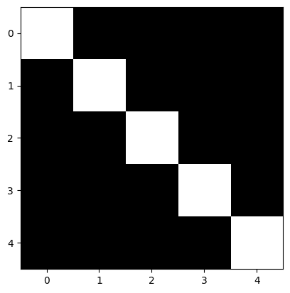
image = np.array([
    [1, 0, 0, 0, 0],
    [0, 1, 0, 0, 0],
    [0, 0, 1, 0, 0],
    [0, 0, 0, 1, 0],
    [0, 0, 0, 0, 1]
])

plt.imshow(image, cmap='gray')
plt.show()

# Example 2x2 kernel
kernel = np.array([
    [1, 0],
    [0, 1]
])

plt.imshow(kernel, cmap='gray')
plt.show()


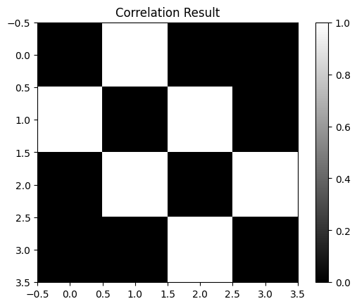
result = correlate2d(image, kernel, mode='valid')
print(result)
plt.imshow(result, cmap='gray')
plt.title('Correlation Result')
plt.colorbar()
plt.show()

[[2 0 0 0]
 [0 2 0 0]
 [0 0 2 0]
 [0 0 0 2]]

Kernel	Pattern Detected	Use Case
[[1,1],[1,1]]	Uniform 2×2 bright block	Detecting blobs or flat regions
[[0,0],[0,0]]	Nothing (zero everywhere)	Theoretical/diagnostic
[[1,0],[0,1]]	Diagonal (top-left to bottom-right)	Detecting / diagonals
[[0,1],[1,0]]	Diagonal (top-right to bottom-left)	Detecting \ diagonals

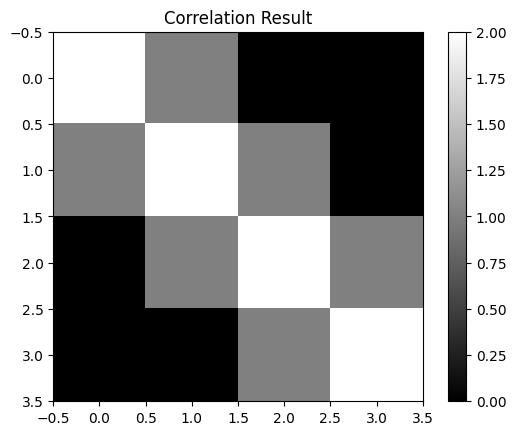
# Example 2x2 kernel
kernel = np.array([
    [1, 1],
    [1, 1]
])

plt.imshow(kernel, cmap='gray')
plt.show()


result = correlate2d(image, kernel, mode='valid')
print(result)
plt.imshow(result, cmap='gray')
plt.title('Correlation Result')
plt.colorbar()
plt.show()

[[2 1 0 0]
 [1 2 1 0]
 [0 1 2 1]
 [0 0 1 2]]

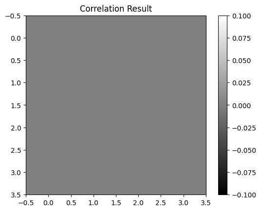
# Example 2x2 kernel
kernel = np.array([
    [0, 0],
    [0, 0]
])

plt.imshow(kernel, cmap='gray')
plt.show()


result = correlate2d(image, kernel, mode='valid')

plt.imshow(result, cmap='gray')
plt.title('Correlation Result')
plt.colorbar()
plt.show()

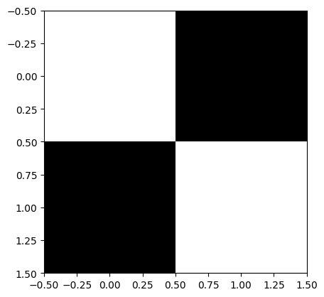
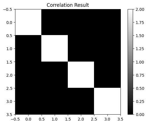
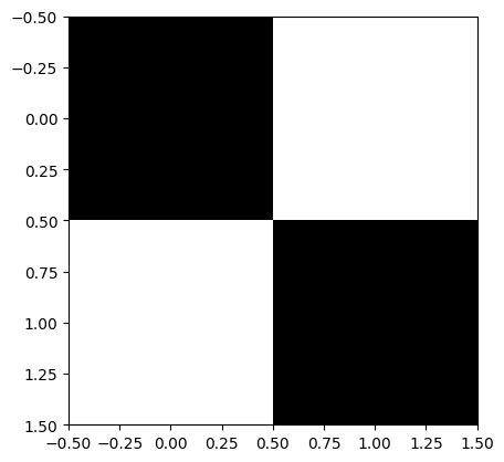
# Example 2x2 kernel
kernel = np.array([
    [0, 1],
    [1, 0]
])

plt.imshow(kernel, cmap='gray')
plt.show()


result = correlate2d(image, kernel, mode='valid')

plt.imshow(result, cmap='gray')
plt.title('Correlation Result')
plt.colorbar()
plt.show()

Max Pooling

MaxPooling2D is an operation in convolutional neural networks (CNNs) that reduces the spatial dimensions (width and height) of feature maps by summarizing local regions.

How MaxPooling2D Works:

Given a feature map, MaxPooling divides it into smaller regions (typically \(2 \times 2\)) and selects the maximum value from each region.

Example:

Suppose we have a \(4 \times 4\) feature map:

\[\begin{split} \begin{bmatrix} 1 & 3 & 2 & 1 \\[6pt] 4 & 6 & 5 & 2 \\[6pt] 7 & 8 & 9 & 3 \\[6pt] 4 & 5 & 2 & 1 \end{bmatrix} \end{split}\]

We apply a MaxPooling operation with a \(2\times2\) pooling region and stride = \(2\). This divides the feature map into four distinct regions:

• Region 1 (top-left):
  $\( \begin{bmatrix} 1 & 3 \\[6pt] 4 & 6 \end{bmatrix} \quad\Rightarrow\quad \max(1, 3, 4, 6) = 6 \)$

• Region 2 (top-right):
  $\( \begin{bmatrix} 2 & 1 \\[6pt] 5 & 2 \end{bmatrix} \quad\Rightarrow\quad \max(2, 1, 5, 2) = 5 \)$

• Region 3 (bottom-left):
  $\( \begin{bmatrix} 7 & 8 \\[6pt] 4 & 5 \end{bmatrix} \quad\Rightarrow\quad \max(7, 8, 4, 5) = 8 \)$

• Region 4 (bottom-right):
  $\( \begin{bmatrix} 9 & 3 \\[6pt] 2 & 1 \end{bmatrix} \quad\Rightarrow\quad \max(9, 3, 2, 1) = 9 \)$

Resulting Feature Map:

After MaxPooling, the resulting feature map is smaller (\(2\times2\)):

\[\begin{split} \begin{bmatrix} 6 & 5 \\[6pt] 8 & 9 \end{bmatrix} \end{split}\]

Why Use MaxPooling2D?

• Reduces complexity by decreasing the dimensions of the feature map.

• Highlights dominant features by keeping the maximum values.

inputs = keras.Input(shape=(28, 28, 1))
x = layers.Conv2D(filters=32, kernel_size=3, activation="relu")(inputs)
x = layers.Conv2D(filters=64, kernel_size=3, activation="relu")(x)
x = layers.Conv2D(filters=128, kernel_size=3, activation="relu")(x)
x = layers.Flatten()(x)
outputs = layers.Dense(10, activation="softmax")(x)

model_no_max_pool = keras.Model(inputs=inputs, outputs=outputs)

from tensorflow.keras.datasets import mnist

(train_images, train_labels), (test_images, test_labels) = mnist.load_data() 

train_images = train_images.reshape((60000, 28, 28, 1))
train_images = train_images.astype("float32") / 255 
test_images = test_images.reshape((10000, 28, 28, 1)) 
test_images = test_images.astype("float32") / 255

model_no_max_pool.compile(optimizer="rmsprop",
              loss="sparse_categorical_crossentropy",
              metrics=["accuracy"])

history = model_no_max_pool.fit(train_images, train_labels, epochs=5, batch_size=64, verbose=0)

test_loss, test_acc = model_no_max_pool.evaluate(test_images, test_labels)
print("Test loss ", test_loss)
print("Test accuracy ", test_acc)

313/313 ━━━━━━━━━━━━━━━━━━━━ 5s 14ms/step - accuracy: 0.9805 - loss: 0.0778
Test loss  0.06550324708223343
Test accuracy  0.9829999804496765