![]()
Loss Functions for Binary Classification#
Before diving into the math, let’s understand why we need to talk about loss functions:
Measuring Success: The loss function tells our model how well (or poorly) it’s performing.
Guiding Improvement: It provides the direction for optimization—like a compass pointing toward better predictions.
Different Problems, Different Tools: Choosing the right loss function can dramatically improve how well and how quickly our model learns.
Binary Cross-Entropy (also known as log loss) is a loss function commonly used for binary classification tasks. It measures the difference between the true labels and the predicted probabilities (usually produced by a sigmoid activation). The binary cross-entropy loss for a single example is given by:
where:
\(y\) is the true label (0 or 1),
\(\hat{y}\) is the predicted probability that the output is 1,
\(\log\) is the natural logarithm.
For a dataset of \(N\) examples, the average loss is:
import numpy as np

# Define binary cross-entropy loss function
def binary_cross_entropy(y_true, y_pred):
    epsilon = 1e-12  # to avoid log(0)
    y_pred = np.clip(y_pred, epsilon, 1 - epsilon)
    loss = -(y_true * np.log(y_pred) + (1 - y_true) * np.log(1 - y_pred))
    return loss

# Example predictions and actual labels
y_true = np.array([0, 1, 1, 0])
y_pred_good = np.array([0.1, 0.9, 0.8, 0.2])  # good predictions
y_pred_bad = np.array([0.9, 0.1, 0.3, 0.8])   # bad predictions

# Calculate losses
loss_good = binary_cross_entropy(y_true, y_pred_good)
loss_bad = binary_cross_entropy(y_true, y_pred_bad)

print("Good Predictions Loss:", loss_good)
print("Average:", np.mean(loss_good))

print("\nBad Predictions Loss:", loss_bad)
print("Average:", np.mean(loss_bad))
Good Predictions Loss: [0.10536052 0.10536052 0.22314355 0.22314355]
Average: 0.164252033486018

Bad Predictions Loss: [2.30258509 2.30258509 1.2039728  1.60943791]
Average: 1.854645225687032
Why Use Binary Cross-Entropy?#
There are several reasons why binary cross-entropy is a popular choice for binary classification tasks:
It Speaks the Language of Probability
Perfect match for sigmoid outputs (0-1 range)
Directly measures the “surprise” of seeing the true label given a prediction
It Punishes Overconfident Mistakes
Being wrong with 99% confidence hurts much more than being wrong with 51% confidence
Creates stronger learning signals when the model makes confident errors
Example: Predicting 0.01 when the true label is 1 creates a massive gradient
It Plays Well with Gradient Descent
Smooth surface with clear gradients throughout the prediction range
No flat spots or sudden drops that could trap or confuse optimization
Mathematically elegant connection to maximum likelihood estimation
Why Other Loss Functions Fall Short#
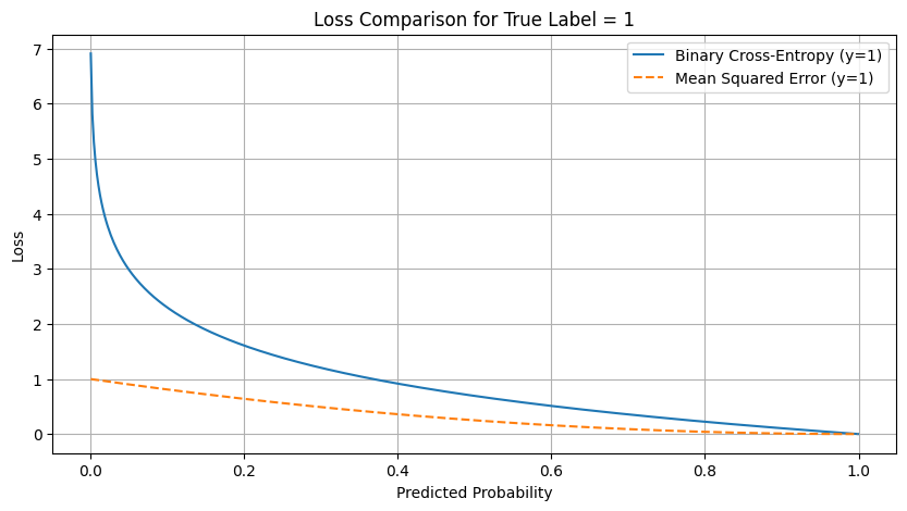
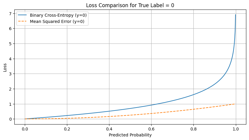
Mean Squared Error (MSE) is given by: $\( \ell_{\text{MSE}}(y, \hat{y}) = (y - \hat{y})^2 \)$
MSE is more commonly used for regression tasks, where the model predicts a continuous value. While it’s possible to use MSE for binary classification, it has several drawbacks:
Designed for continuous values, not binary outcomes
Gradients become weaker for very wrong predictions
In practical terms: MSE cares more about being “in the ballpark” than being exactly right
Hinge Loss is another loss function used for binary classification, especially in the context of Support Vector Machines (SVMs). It is defined as: $\( \ell_{\text{hinge}}(y, \hat{y}) = \max(0, 1 - y \cdot \hat{y}) \)$
Hinge loss is designed to work well with classifiers that aim to maximize the margin between classes. However, it has some limitations:
Not as intuitive when the model outputs probabilities: Doesn’t distinguish between probabilities of 0.51 and 0.99
Non-smooth points in the loss function can make optimization more challenging
import numpy as np
import matplotlib.pyplot as plt

# Define binary cross-entropy loss
def binary_cross_entropy(y_true, y_pred):
    epsilon = 1e-12
    y_pred = np.clip(y_pred, epsilon, 1 - epsilon)
    return -(y_true * np.log(y_pred) + (1 - y_true) * np.log(1 - y_pred))

# Define mean squared error loss
def mse_loss(y_true, y_pred):
    return (y_true - y_pred)**2


# Generate predicted probabilities from 0 to 1
y_pred = np.linspace(0.001, 0.999, 500)

# True label (1)
y_true_1 = 1
bce_loss_1 = binary_cross_entropy(y_true_1, y_pred)
mse_loss_1 = mse_loss(y_true_1, y_pred)

# True label (0)
y_true_0 = 0
bce_loss_0 = binary_cross_entropy(y_true_0, y_pred)
mse_loss_0 = mse_loss(y_true_0, y_pred)

# Plot losses for y_true = 1
plt.figure(figsize=(10,5))
plt.plot(y_pred, bce_loss_1, label='Binary Cross-Entropy (y=1)')
plt.plot(y_pred, mse_loss_1, label='Mean Squared Error (y=1)', linestyle='--')
plt.xlabel("Predicted Probability")
plt.ylabel("Loss")
plt.title("Loss Comparison for True Label = 1")
plt.legend()
plt.grid(True)
plt.show()

# Plot losses for y_true = 0
plt.figure(figsize=(10, 5))
plt.plot(y_pred, bce_loss_0, label='Binary Cross-Entropy (y=0)')
plt.plot(y_pred, mse_loss_0, label='Mean Squared Error (y=0)', linestyle='--')
plt.xlabel("Predicted Probability")
plt.ylabel("Loss")
plt.title("Loss Comparison for True Label = 0")
plt.legend()
plt.grid(True)
plt.show()
import numpy as np
import matplotlib.pyplot as plt
import seaborn as sns
from tensorflow.keras.models import Sequential
from tensorflow.keras.layers import Dense, Input
from tensorflow.keras.optimizers import SGD

# Define the XOR dataset
X = np.array([
    [0, 0],
    [0, 1],
    [1, 0],
    [1, 1]
])
# XOR outputs: 0 if inputs are the same, 1 if they are different
y = np.array([0, 1, 1, 0])

# Create a simple neural network with one hidden layer
model = Sequential([
    Input(shape=(2,)),
    Dense(3, activation='tanh'),  # Hidden layer with 3 neurons using tanh activation
    Dense(1, activation='sigmoid')  # Output layer with sigmoid activation
])

# Compile the model with learning rate of 0.1
optimizer = SGD(learning_rate=0.1)
model.compile(loss='binary_crossentropy', optimizer=optimizer, metrics=['accuracy'])

# Train the model and save the history to track loss over epochs
history = model.fit(X, y, epochs=5000, verbose=0)

# Evaluate the model on the XOR dataset
loss, accuracy = model.evaluate(X, y, verbose=0)
predictions = model.predict(X)
rounded_predictions = np.round(predictions)

print(f"Final loss: {loss:.4f}")
print(f"Final accuracy: {accuracy:.4f}")
print("\nRaw predictions on the XOR dataset:")
for i, pred in enumerate(predictions):
    print(f"Input: {X[i]} → Prediction: {pred[0]:.4f} → Rounded: {rounded_predictions[i][0]}")

# Visualize the loss over epochs
plt.figure(figsize=(10, 6))
plt.plot(history.history['loss'])
plt.title('Model Loss During Training')
plt.ylabel('Binary Crossentropy Loss')
plt.xlabel('Epoch')
plt.grid(True)
sns.despine()
plt.show()

# Optional: Create a decision boundary visualization
plt.figure(figsize=(10, 6))

# Create a grid of points
h = 0.01
x_min, x_max = -0.5, 1.5
y_min, y_max = -0.5, 1.5
xx, yy = np.meshgrid(np.arange(x_min, x_max, h), np.arange(y_min, y_max, h))
grid_points = np.c_[xx.ravel(), yy.ravel()]

# Get predictions for all grid points
Z = model.predict(grid_points)
Z = Z.reshape(xx.shape)

# Plot the decision boundary
plt.contourf(xx, yy, Z, cmap=plt.cm.RdBu, alpha=0.8)

# Plot the training points
plt.scatter(X[:, 0], X[:, 1], c=y, edgecolors='k', cmap=plt.cm.RdBu)
plt.xlim(xx.min(), xx.max())
plt.ylim(yy.min(), yy.max())
plt.xlabel('Input 1')
plt.ylabel('Input 2')
plt.title('XOR Decision Boundary')
plt.colorbar()
plt.grid(True)

plt.show()
2025-05-08 15:01:47.636799: I external/local_xla/xla/tsl/cuda/cudart_stub.cc:32] Could not find cuda drivers on your machine, GPU will not be used.
2025-05-08 15:01:47.640023: I external/local_xla/xla/tsl/cuda/cudart_stub.cc:32] Could not find cuda drivers on your machine, GPU will not be used.
2025-05-08 15:01:47.653384: E external/local_xla/xla/stream_executor/cuda/cuda_fft.cc:467] Unable to register cuFFT factory: Attempting to register factory for plugin cuFFT when one has already been registered
WARNING: All log messages before absl::InitializeLog() is called are written to STDERR
E0000 00:00:1746716507.667452   29243 cuda_dnn.cc:8579] Unable to register cuDNN factory: Attempting to register factory for plugin cuDNN when one has already been registered
E0000 00:00:1746716507.671542   29243 cuda_blas.cc:1407] Unable to register cuBLAS factory: Attempting to register factory for plugin cuBLAS when one has already been registered
W0000 00:00:1746716507.683046   29243 computation_placer.cc:177] computation placer already registered. Please check linkage and avoid linking the same target more than once.
W0000 00:00:1746716507.683057   29243 computation_placer.cc:177] computation placer already registered. Please check linkage and avoid linking the same target more than once.
W0000 00:00:1746716507.683058   29243 computation_placer.cc:177] computation placer already registered. Please check linkage and avoid linking the same target more than once.
W0000 00:00:1746716507.683060   29243 computation_placer.cc:177] computation placer already registered. Please check linkage and avoid linking the same target more than once.
2025-05-08 15:01:47.687150: I tensorflow/core/platform/cpu_feature_guard.cc:210] This TensorFlow binary is optimized to use available CPU instructions in performance-critical operations.
To enable the following instructions: AVX2 FMA, in other operations, rebuild TensorFlow with the appropriate compiler flags.
2025-05-08 15:01:49.294496: E external/local_xla/xla/stream_executor/cuda/cuda_platform.cc:51] failed call to cuInit: INTERNAL: CUDA error: Failed call to cuInit: UNKNOWN ERROR (303)
---------------------------------------------------------------------------
KeyboardInterrupt                         Traceback (most recent call last)
Cell In[3], line 30
     27 model.compile(loss='binary_crossentropy', optimizer=optimizer, metrics=['accuracy'])
     29 # Train the model and save the history to track loss over epochs
---> 30 history = model.fit(X, y, epochs=5000, verbose=0)
     32 # Evaluate the model on the XOR dataset
     33 loss, accuracy = model.evaluate(X, y, verbose=0)

File /opt/hostedtoolcache/Python/3.11.12/x64/lib/python3.11/site-packages/keras/src/utils/traceback_utils.py:117, in filter_traceback.<locals>.error_handler(*args, **kwargs)
    115 filtered_tb = None
    116 try:
--> 117     return fn(*args, **kwargs)
    118 except Exception as e:
    119     filtered_tb = _process_traceback_frames(e.__traceback__)

File /opt/hostedtoolcache/Python/3.11.12/x64/lib/python3.11/site-packages/keras/src/backend/tensorflow/trainer.py:371, in TensorFlowTrainer.fit(self, x, y, batch_size, epochs, verbose, callbacks, validation_split, validation_data, shuffle, class_weight, sample_weight, initial_epoch, steps_per_epoch, validation_steps, validation_batch_size, validation_freq)
    369 for step, iterator in epoch_iterator:
    370     callbacks.on_train_batch_begin(step)
--> 371     logs = self.train_function(iterator)
    372     callbacks.on_train_batch_end(step, logs)
    373     if self.stop_training:

File /opt/hostedtoolcache/Python/3.11.12/x64/lib/python3.11/site-packages/keras/src/backend/tensorflow/trainer.py:219, in TensorFlowTrainer._make_function.<locals>.function(iterator)
    215 def function(iterator):
    216     if isinstance(
    217         iterator, (tf.data.Iterator, tf.distribute.DistributedIterator)
    218     ):
--> 219         opt_outputs = multi_step_on_iterator(iterator)
    220         if not opt_outputs.has_value():
    221             raise StopIteration

File /opt/hostedtoolcache/Python/3.11.12/x64/lib/python3.11/site-packages/tensorflow/python/util/traceback_utils.py:150, in filter_traceback.<locals>.error_handler(*args, **kwargs)
    148 filtered_tb = None
    149 try:
--> 150   return fn(*args, **kwargs)
    151 except Exception as e:
    152   filtered_tb = _process_traceback_frames(e.__traceback__)

File /opt/hostedtoolcache/Python/3.11.12/x64/lib/python3.11/site-packages/tensorflow/python/eager/polymorphic_function/polymorphic_function.py:833, in Function.__call__(self, *args, **kwds)
    830 compiler = "xla" if self._jit_compile else "nonXla"
    832 with OptionalXlaContext(self._jit_compile):
--> 833   result = self._call(*args, **kwds)
    835 new_tracing_count = self.experimental_get_tracing_count()
    836 without_tracing = (tracing_count == new_tracing_count)

File /opt/hostedtoolcache/Python/3.11.12/x64/lib/python3.11/site-packages/tensorflow/python/eager/polymorphic_function/polymorphic_function.py:878, in Function._call(self, *args, **kwds)
    875 self._lock.release()
    876 # In this case we have not created variables on the first call. So we can
    877 # run the first trace but we should fail if variables are created.
--> 878 results = tracing_compilation.call_function(
    879     args, kwds, self._variable_creation_config
    880 )
    881 if self._created_variables:
    882   raise ValueError("Creating variables on a non-first call to a function"
    883                    " decorated with tf.function.")

File /opt/hostedtoolcache/Python/3.11.12/x64/lib/python3.11/site-packages/tensorflow/python/eager/polymorphic_function/tracing_compilation.py:139, in call_function(args, kwargs, tracing_options)
    137 bound_args = function.function_type.bind(*args, **kwargs)
    138 flat_inputs = function.function_type.unpack_inputs(bound_args)
--> 139 return function._call_flat(  # pylint: disable=protected-access
    140     flat_inputs, captured_inputs=function.captured_inputs
    141 )

File /opt/hostedtoolcache/Python/3.11.12/x64/lib/python3.11/site-packages/tensorflow/python/eager/polymorphic_function/concrete_function.py:1322, in ConcreteFunction._call_flat(self, tensor_inputs, captured_inputs)
   1318 possible_gradient_type = gradients_util.PossibleTapeGradientTypes(args)
   1319 if (possible_gradient_type == gradients_util.POSSIBLE_GRADIENT_TYPES_NONE
   1320     and executing_eagerly):
   1321   # No tape is watching; skip to running the function.
-> 1322   return self._inference_function.call_preflattened(args)
   1323 forward_backward = self._select_forward_and_backward_functions(
   1324     args,
   1325     possible_gradient_type,
   1326     executing_eagerly)
   1327 forward_function, args_with_tangents = forward_backward.forward()

File /opt/hostedtoolcache/Python/3.11.12/x64/lib/python3.11/site-packages/tensorflow/python/eager/polymorphic_function/atomic_function.py:216, in AtomicFunction.call_preflattened(self, args)
    214 def call_preflattened(self, args: Sequence[core.Tensor]) -> Any:
    215   """Calls with flattened tensor inputs and returns the structured output."""
--> 216   flat_outputs = self.call_flat(*args)
    217   return self.function_type.pack_output(flat_outputs)

File /opt/hostedtoolcache/Python/3.11.12/x64/lib/python3.11/site-packages/tensorflow/python/eager/polymorphic_function/atomic_function.py:251, in AtomicFunction.call_flat(self, *args)
    249 with record.stop_recording():
    250   if self._bound_context.executing_eagerly():
--> 251     outputs = self._bound_context.call_function(
    252         self.name,
    253         list(args),
    254         len(self.function_type.flat_outputs),
    255     )
    256   else:
    257     outputs = make_call_op_in_graph(
    258         self,
    259         list(args),
    260         self._bound_context.function_call_options.as_attrs(),
    261     )

File /opt/hostedtoolcache/Python/3.11.12/x64/lib/python3.11/site-packages/tensorflow/python/eager/context.py:1688, in Context.call_function(self, name, tensor_inputs, num_outputs)
   1686 cancellation_context = cancellation.context()
   1687 if cancellation_context is None:
-> 1688   outputs = execute.execute(
   1689       name.decode("utf-8"),
   1690       num_outputs=num_outputs,
   1691       inputs=tensor_inputs,
   1692       attrs=attrs,
   1693       ctx=self,
   1694   )
   1695 else:
   1696   outputs = execute.execute_with_cancellation(
   1697       name.decode("utf-8"),
   1698       num_outputs=num_outputs,
   (...)   1702       cancellation_manager=cancellation_context,
   1703   )

File /opt/hostedtoolcache/Python/3.11.12/x64/lib/python3.11/site-packages/tensorflow/python/eager/execute.py:53, in quick_execute(op_name, num_outputs, inputs, attrs, ctx, name)
     51 try:
     52   ctx.ensure_initialized()
---> 53   tensors = pywrap_tfe.TFE_Py_Execute(ctx._handle, device_name, op_name,
     54                                       inputs, attrs, num_outputs)
     55 except core._NotOkStatusException as e:
     56   if name is not None:

KeyboardInterrupt:
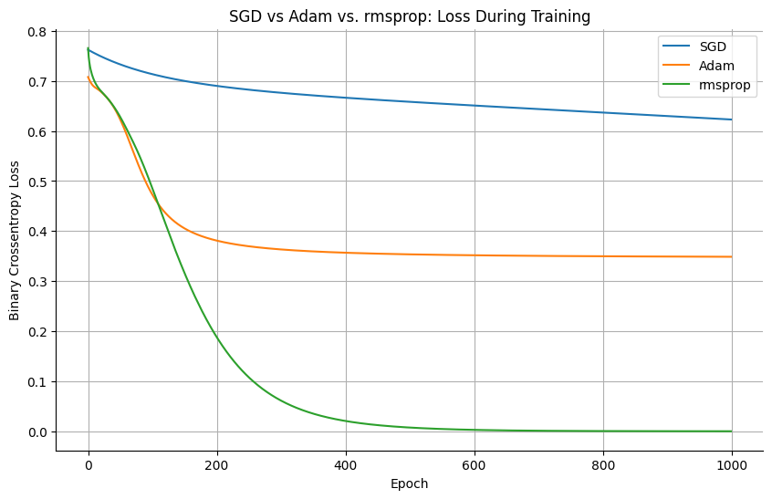
Brief Discussion of Optimizers#
Keras provides several built-in optimizers that adjust the model parameters during training. In addition to the classic Stochastic Gradient Descent (SGD), there are more advanced optimizers like adam or rmsprop.
# Compare SGD with Adam optimizer
from tensorflow.keras.optimizers import SGD, Adam, RMSprop
import matplotlib.pyplot as plt
import seaborn as sns

# Function to train model with different optimizers
def train_with_optimizer(optimizer_name):
    # Reset the model
    model = Sequential([
        Input(shape=(2,)),
        Dense(3, activation='tanh'),
        Dense(1, activation='sigmoid')
    ])

    # Select optimizer
    if optimizer_name == 'SGD':
        opt = SGD(learning_rate=0.01)
    elif optimizer_name == "Adam":
        opt = Adam(learning_rate=0.01)
    elif optimizer_name == "RMSprop":
        opt = RMSprop(learning_rate=0.01)

    model.compile(loss='binary_crossentropy', optimizer=opt)

    # Train and record history
    history = model.fit(X, y, epochs=1000, verbose=0)
    return history.history['loss']

# Train with both optimizers
sgd_loss = train_with_optimizer('SGD')
adam_loss = train_with_optimizer('Adam')
rmsprop_loss = train_with_optimizer('RMSprop')

# Plot comparison
plt.figure(figsize=(10, 6))
plt.plot(sgd_loss, label='SGD')
plt.plot(adam_loss, label='Adam')
plt.plot(rmsprop_loss, label='rmsprop')
plt.title('SGD vs Adam vs. rmsprop: Loss During Training')
plt.ylabel('Binary Crossentropy Loss')
plt.xlabel('Epoch')
plt.legend()
sns.despine()
plt.grid(True)
plt.show()