A Brief Introduction to Numpy

A Brief Introduction to Numpy#

Numpy is a Python library that provides support for large, multi-dimensional arrays and matrices, along with a collection of mathematical functions to operate on these arrays. It is the fundamental package for scientific computing with Python.

In this notebook, we will cover the following topics:

Creating Numpy arrays
Basic operations on Numpy arrays
Indexing and slicing
Reshaping and resizing
Stacking and splitting
Broadcasting

import numpy as np

x = np.array([1, 2, 3.0, 4, 5]) # 1-dimensional array
print(x)
print("Number of dimensions: ", x.ndim) # the number of dimensions
print("The datatype of x is: ", x.dtype) # the datatype of the array
print("Shape: ", x.shape) # the shape of the array: a tuple of the size of each dimension
print("Size: ", x.size) # the size is the number of elements in the array

[1. 2. 3. 4. 5.]
Number of dimensions:  1
The datatype of x is:  float64
Shape:  (5,)
Size:  5

x = np.array(7) # scalar
print(x)
print("Number of dimensions: ", x.ndim) # the number of dimensions
print("Shape: ", x.shape) # the shape of the array: a tuple of the size of each dimension
print("Size: ", x.size) # the size is the number of elements in the array
print("The datatype of the array: ", x.dtype) # the datatype of the array

7
Number of dimensions:  0
Shape:  ()
Size:  1
The datatype of the array:  int64

x = np.array([[1, 2, 3], [4, 5, 6], [7, 8, 9]]) # 2-dimensional array
print(x)
print("Number of dimensions: ", x.ndim) # the number of dimensions
print("Shape: ", x.shape) # the shape of the array: a tuple of the size of each dimension
print("Size: ", x.size) # the size is the number of elements in the array
print("The datatype of the array: ", x.dtype) # the datatype of the array

[[1 2 3]
 [4 5 6]
 [7 8 9]]
Number of dimensions:  2
Shape:  (3, 3)
Size:  9
The datatype of the array:  int64

x = np.array([[[1, 2], [3, 4]], [[5, 6], [7, 8]]]) # 3-dimensional array
print(x)
print("Number of dimensions: ", x.ndim) # the number of dimensions
print("Shape: ", x.shape) # the shape of the array: a tuple of the size of each dimension
print("Size: ", x.size) # the size is the number of elements in the array
print("The datatype of the array: ", x.dtype) # the datatype of the array

[[[1 2]
  [3 4]]

 [[5 6]
  [7 8]]]
Number of dimensions:  3
Shape:  (2, 2, 2)
Size:  8
The datatype of the array:  int64

Creating Numpy arrays#

# Create an array from a list
arr_list = np.array([1, 2, 3])
print("Array from list:\n", arr_list)
print("The datatype of the array: ", arr_list.dtype) 
# Create an array of zeros
arr_zeros = np.zeros((3, 2))
print("\nArray of zeros:\n", arr_zeros)
print("The datatype of the array: ", arr_zeros.dtype) 

# Create an array of ones
arr_ones = np.ones((3, 2))
print("\nArray of ones:\n", arr_ones)
print("The datatype of the array: ", arr_ones.dtype)

# Create an array filled with a specific value
arr_full = np.full((3, 2), 7)
print("\nArray filled with 7:\n", arr_full)
print("The datatype of the array: ", arr_full.dtype)

# Create an array with a range of values
arr_range = np.arange(0, 10, 2)
print("\nArray with range values:\n", arr_range)
print("The datatype of the array: ", arr_range.dtype)

# Create an array with evenly spaced values
arr_linspace = np.linspace(0, 1, 5)
print("\nArray with evenly spaced values:\n", arr_linspace)
print("The datatype of the array: ", arr_linspace.dtype)

# Create an array with random values
arr_random = np.random.rand(3, 3)
print("\nArray with random values:\n", arr_random)
print("The datatype of the array: ", arr_random.dtype)

Array from list:
 [1 2 3]
The datatype of the array:  int64

Array of zeros:
 [[0. 0.]
 [0. 0.]
 [0. 0.]]
The datatype of the array:  float64

Array of ones:
 [[1. 1.]
 [1. 1.]
 [1. 1.]]
The datatype of the array:  float64

Array filled with 7:
 [[7 7]
 [7 7]
 [7 7]]
The datatype of the array:  int64

Array with range values:
 [0 2 4 6 8]
The datatype of the array:  int64

Array with evenly spaced values:
 [0.   0.25 0.5  0.75 1.  ]
The datatype of the array:  float64

Array with random values:
 [[0.00726373 0.108089   0.7383138 ]
 [0.76552    0.53744706 0.49445693]
 [0.50851987 0.28503847 0.42879653]]
The datatype of the array:  float64

Indexing and slicing#

# Create a sample 1D array
arr_1d = np.array([10, 20, 30, 40, 50])
print("1D Array:\n", arr_1d)

# Access the first element
print("\nFirst element of 1D array:", arr_1d[0])

# Create a sample 2D array
arr_2d = np.array([
    [1, 2, 3],
    [4, 5, 6],
    [7, 8, 9]
])
print("\n2D Array:\n", arr_2d)

# Access an element in a multi-dimensional array
print("\nElement at row index 1, column index 2:", arr_2d[1, 2])

# Slice all rows, second column
print("\nAll rows, second column:\n", arr_2d[:, 1])

# Slice elements from index 1 to 3 in a 1D array
print("\nSlice from index 1 to 3 in 1D array:", arr_1d[1:4])

1D Array:
 [10 20 30 40 50]

First element of 1D array: 10

2D Array:
 [[1 2 3]
 [4 5 6]
 [7 8 9]]

Element at row index 1, column index 2: 6

All rows, second column:
 [2 5 8]

Slice from index 1 to 3 in 1D array: [20 30 40]

# Create a sample 2D array
arr_2d = np.array([
    [10, 20, 30],
    [40, 50, 60],
    [70, 80, 90]
])
print("2D Array:\n", arr_2d, "\nShape:", arr_2d.shape)

# Select all rows, second column
slice_1 = arr_2d[:, 1]
print("\nAll rows, second column:\n", slice_1, "\nShape:", slice_1.shape)

# Select all rows, last column
slice_2 = arr_2d[:, -1]
print("\nAll rows, last column:\n", slice_2, "\nShape:", slice_2.shape)

# Select first row, all columns
slice_3 = arr_2d[0, :]
print("\nFirst row, all columns:\n", slice_3, "\nShape:", slice_3.shape)

# Select first two rows, all columns
slice_4 = arr_2d[:2, :]
print("\nFirst two rows, all columns:\n", slice_4, "\nShape:", slice_4.shape)

# Select bottom-right 2x2 subarray
slice_5 = arr_2d[1:, 1:]
print("\nBottom-right 2x2 subarray:\n", slice_5, "\nShape:", slice_5.shape)

2D Array:
 [[10 20 30]
 [40 50 60]
 [70 80 90]] 
Shape: (3, 3)

All rows, second column:
 [20 50 80] 
Shape: (3,)

All rows, last column:
 [30 60 90] 
Shape: (3,)

First row, all columns:
 [10 20 30] 
Shape: (3,)

First two rows, all columns:
 [[10 20 30]
 [40 50 60]] 
Shape: (2, 3)

Bottom-right 2x2 subarray:
 [[50 60]
 [80 90]] 
Shape: (2, 2)

More on reshaping arrays#

# Create a sample 2D array
arr = np.array([
    [1, 2, 3],
    [4, 5, 6],
    [7, 8, 9],
    [10, 11, 12]
])

print("Original Array:\n", arr)
print("Shape of original array:", arr.shape)

# Reshape to 1D (flattening)
arr_1d = arr.reshape(-1)
print("\nReshaped to 1D:\n", arr_1d)
print("Shape:", arr_1d.shape)

# Reshape to 2D (2 rows, 6 columns)
arr_2d = arr.reshape(2, 6)
print("\nReshaped to 2D (2x6):\n", arr_2d)
print("Shape:", arr_2d.shape)

# Reshape to 3D (2 blocks, 2 rows, 3 columns)
arr_3d = arr.reshape(2, 2, 3)
print("\nReshaped to 3D (2x2x3):\n", arr_3d)
print("Shape:", arr_3d.shape)

# Example of an invalid reshape (will cause an error)
try:
    arr_invalid = arr.reshape(3, 5)  # 12 elements cannot fit into a (3x5) shape
    print("\nReshaped to 3x5:\n", arr_invalid)
except ValueError as e:
    print("\nInvalid reshape (3x5) failed with error:", e)

Original Array:
 [[ 1  2  3]
 [ 4  5  6]
 [ 7  8  9]
 [10 11 12]]
Shape of original array: (4, 3)

Reshaped to 1D:
 [ 1  2  3  4  5  6  7  8  9 10 11 12]
Shape: (12,)

Reshaped to 2D (2x6):
 [[ 1  2  3  4  5  6]
 [ 7  8  9 10 11 12]]
Shape: (2, 6)

Reshaped to 3D (2x2x3):
 [[[ 1  2  3]
  [ 4  5  6]]

 [[ 7  8  9]
  [10 11 12]]]
Shape: (2, 2, 3)

Invalid reshape (3x5) failed with error: cannot reshape array of size 12 into shape (3,5)

NumPy `reshape` Summary#

The reshape function is used to give a new shape to an array without changing its data. The reshape function returns a new array object with the new shape specified by the parameters (tuple of integers). The new shape should be compatible with the original shape. If an integer in the reshape function is set to -1, the value is inferred from the length of the array and remaining dimensions.

Command	Effect	Shape Example
`reshape(-1)`	Flattens to a 1D array	`(n,)`
`reshape(1, -1)`	Converts to a row vector (1 row, many cols)	`(1, n)`
`reshape(-1, 1)`	Converts to a column vector (many rows, 1 col)	`(n, 1)`
`reshape(1)`	❌ Invalid unless the array has only 1 element	N/A

# Create a 3D array (2 blocks, 2 rows, 3 columns)
arr_3d = np.array([
    [[1, 2, 3], [4, 5, 6]],
    [[7, 8, 9], [10, 11, 12]]
])

print("Original 3D Array:\n", arr_3d)
print("Shape:", arr_3d.shape)  # (2, 2, 3)

# Flatten the 3D array
arr_flattened = arr_3d.reshape(-1)
print("\nFlattened Array:\n", arr_flattened)
print("Shape after flattening:", arr_flattened.shape)  # (12,)

Original 3D Array:
 [[[ 1  2  3]
  [ 4  5  6]]

 [[ 7  8  9]
  [10 11 12]]]
Shape: (2, 2, 3)

Flattened Array:
 [ 1  2  3  4  5  6  7  8  9 10 11 12]
Shape after flattening: (12,)

Stacking and concatenating arrays#

import numpy as np

# Create two sample arrays
arr1 = np.array([
    [1, 2, 3],
    [4, 5, 6]
])

arr2 = np.array([
    [7, 8, 9],
    [10, 11, 12]
])

print("Array 1:\n", arr1)
print("Shape of arr1:", arr1.shape)

print("\nArray 2:\n", arr2)
print("Shape of arr2:", arr2.shape)

# Concatenate along axis 0 (rows)
concatenated_0 = np.concatenate((arr1, arr2), axis=0)
print("\nConcatenated along axis 0 (rows):\n", concatenated_0)
print("Shape:", concatenated_0.shape)

# Concatenate along axis 1 (columns)
concatenated_1 = np.concatenate((arr1, arr2), axis=1)
print("\nConcatenated along axis 1 (columns):\n", concatenated_1)
print("Shape:", concatenated_1.shape)

# Stack vertically (equivalent to axis=0 concatenation)
stacked_v = np.vstack((arr1, arr2))
print("\nStacked Vertically:\n", stacked_v)
print("Shape:", stacked_v.shape)

# Stack horizontally (equivalent to axis=1 concatenation)
stacked_h = np.hstack((arr1, arr2))
print("\nStacked Horizontally:\n", stacked_h)
print("Shape:", stacked_h.shape)

Array 1:
 [[1 2 3]
 [4 5 6]]
Shape of arr1: (2, 3)

Array 2:
 [[ 7  8  9]
 [10 11 12]]
Shape of arr2: (2, 3)

Concatenated along axis 0 (rows):
 [[ 1  2  3]
 [ 4  5  6]
 [ 7  8  9]
 [10 11 12]]
Shape: (4, 3)

Concatenated along axis 1 (columns):
 [[ 1  2  3  7  8  9]
 [ 4  5  6 10 11 12]]
Shape: (2, 6)

Stacked Vertically:
 [[ 1  2  3]
 [ 4  5  6]
 [ 7  8  9]
 [10 11 12]]
Shape: (4, 3)

Stacked Horizontally:
 [[ 1  2  3  7  8  9]
 [ 4  5  6 10 11 12]]
Shape: (2, 6)

Arithmetic operations#

It is important to note that arithmetic operations on arrays are element-wise. This means that the operation is applied to each element of the array.

# Create two sample arrays
arr = np.array([
    [1, 2, 3],
    [4, 5, 6]
])

arr1 = np.array([
    [1, 2, 3],
    [4, 5, 6]
])

arr2 = np.array([
    [7, 8, 9],
    [10, 11, 12]
])

print("Array:\n", arr)

# Add a scalar to all elements
arr_add_scalar = arr + 2
print("\nArray + 2:\n", arr_add_scalar)

# Element-wise addition
arr_add = arr1 + arr2
print("\nElement-wise Addition (arr1 + arr2):\n", arr_add)

# Apply mathematical functions element-wise
arr_exp = np.exp(arr)
print("\nExponential Function (np.exp(arr)):\n", arr_exp)

arr_sin = np.sin(arr)
print("\nSine Function (np.sin(arr)):\n", arr_sin)

arr_log = np.log(arr + 1)  # Adding 1 to avoid log(0)
print("\nLogarithm Function (np.log(arr + 1)):\n", arr_log)

Array:
 [[1 2 3]
 [4 5 6]]

Array + 2:
 [[3 4 5]
 [6 7 8]]

Element-wise Addition (arr1 + arr2):
 [[ 8 10 12]
 [14 16 18]]

Exponential Function (np.exp(arr)):
 [[  2.71828183   7.3890561   20.08553692]
 [ 54.59815003 148.4131591  403.42879349]]

Sine Function (np.sin(arr)):
 [[ 0.84147098  0.90929743  0.14112001]
 [-0.7568025  -0.95892427 -0.2794155 ]]

Logarithm Function (np.log(arr + 1)):
 [[0.69314718 1.09861229 1.38629436]
 [1.60943791 1.79175947 1.94591015]]

Multiplication#

# Create two 1D arrays
arr1 = np.array([1, 2, 3])
arr2 = np.array([4, 5, 6])

print("1D Array 1:", arr1)
print("1D Array 2:", arr2)

# Scalar multiplication
arr1_scalar = arr1 * 3
print("\nScalar Multiplication (arr1 * 3):", arr1_scalar)

# Element-wise multiplication
arr1_elementwise = arr1 * arr2
print("\nElement-wise Multiplication (arr1 * arr2):", arr1_elementwise)

# Dot product of 1D arrays
arr1_dot = np.dot(arr1, arr2)  # Equivalent to sum(arr1 * arr2)
print("\nDot Product (arr1 dot arr2):", arr1_dot)

# Alternative syntax for dot product using @ operator 
arr1_dot_alt = arr1 @ arr2
print("\nDot Product using @ operator:", arr1_dot_alt)

1D Array 1: [1 2 3]
1D Array 2: [4 5 6]

Scalar Multiplication (arr1 * 3): [3 6 9]

Element-wise Multiplication (arr1 * arr2): [ 4 10 18]

Dot Product (arr1 dot arr2): 32

Dot Product using @ operator: 32

# Create two sample arrays

arr1 = np.array([
    [1, 2, 3],
    [4, 5, 6]
])

arr2 = np.array([
    [7, 8, 9],
    [10, 11, 12]
])

print("Array 1:\n", arr1)
print("\nArray 2:\n", arr2)

# Scalar multiplication
arr_mul_scalar = arr1 * 3
print("\nScalar Multiplication (arr * 3):\n", arr_mul_scalar)

# Element-wise multiplication
arr_mul_elementwise = arr1 * arr2
print("\nElement-wise Multiplication (arr1 * arr2):\n", arr_mul_elementwise)

# Matrix multiplication (dot product)
arr_dot = np.dot(arr1, arr2.T)  # Using transpose to match dimensions
print("\nMatrix Multiplication (arr1 dot arr2.T):\n", arr_dot)
print("\nMatrix Multiplication (arr1 @ arr2.T):\n", arr1 @ arr2.T)

Array 1:
 [[1 2 3]
 [4 5 6]]

Array 2:
 [[ 7  8  9]
 [10 11 12]]

Scalar Multiplication (arr * 3):
 [[ 3  6  9]
 [12 15 18]]

Element-wise Multiplication (arr1 * arr2):
 [[ 7 16 27]
 [40 55 72]]

Matrix Multiplication (arr1 dot arr2.T):
 [[ 50  68]
 [122 167]]

Matrix Multiplication (arr1 @ arr2.T):
 [[ 50  68]
 [122 167]]

Broadcasting#

Broadcasting in NumPy allows operations between arrays of different shapes without explicit duplication. NumPy follows three fundamental rules:

Rule 1: Match Dimensions from Right to Left

NumPy aligns array shapes starting from the last dimension.
If the dimensions match or one of them is 1, broadcasting can proceed.
If dimensions don’t match and neither is 1, broadcasting fails.

Rule 2: Expand Dimensions When 1 is Present

If a dimension is 1, NumPy stretches it to match the other array.

Rule 3: Arrays Must Have Compatible Shapes

After applying Rules 1 & 2, the final shapes must match.
If after expansion, shapes remain incompatible, broadcasting fails.

Scenario	Example Shapes	Broadcastable?	Why?
Scalar + Array	`() + (3, 3)`	✅ Yes	Scalar expands to `(3,3)`
1D + 2D (aligned)	`(3,) + (3,3)`	✅ Yes	`(3,)` is treated as `(1,3)` and expands to `(3,3)`
Column Vector + 2D	`(3,1) + (3,3)`	✅ Yes	`(3,1)` expands across columns
Row Vector + 2D	`(1,3) + (3,3)`	✅ Yes	`(1,3)` expands across rows
Mismatched Shapes	`(3,4) + (3,2)`	❌ No	Final shapes do not match

# Rule 1: Match dimensions from right to left
A = np.array([[1, 2, 3], [4, 5, 6]])  # Shape (2,3)
B = np.array([10, 20, 30])  # Shape (3,)
print("A:\n", A)
print("\nB:\n", B)
print("\nBroadcasting Example (A + B):\n", A + B)  # B is expanded to (2,3)

# Rule 2: Expand dimensions when `1` is present (Column Vector)
C = np.array([[10], [20]])  # Shape (2,1)
print("\nC:\n", C)
print("\nBroadcasting Column Vector (A + C):\n", A + C)  # C expands to (2,3)

# Rule 2: Expand dimensions when `1` is present (Row Vector)
D = np.array([[10, 20, 30]])  # Shape (1,3)
print("\nD:\n", D)
print("\nBroadcasting Row Vector (A + D):\n", A + D)  # D expands to (2,3)

# Rule 3: Example where broadcasting fails
E = np.array([[1, 2], [3, 4]])  # Shape (2,2)
print("\nE:\n", E)
try:
    print("\nBroadcasting Error Example (A + E):")
    print(A + E)  # Broadcasting fails because shapes (2,3) and (2,2) are incompatible
except ValueError as e:
    print("Error:", e)

A:
 [[1 2 3]
 [4 5 6]]

B:
 [10 20 30]

Broadcasting Example (A + B):
 [[11 22 33]
 [14 25 36]]

C:
 [[10]
 [20]]

Broadcasting Column Vector (A + C):
 [[11 12 13]
 [24 25 26]]

D:
 [[10 20 30]]

Broadcasting Row Vector (A + D):
 [[11 22 33]
 [14 25 36]]

E:
 [[1 2]
 [3 4]]

Broadcasting Error Example (A + E):
Error: operands could not be broadcast together with shapes (2,3) (2,2) 

Boolean Operations#

# Create a sample array
arr = np.array([
    [1, 5, 7],
    [8, 3, 6]
])

print("Original Array:\n", arr)

# 1. Boolean mask: Check which elements are greater than 5
bool_mask = arr > 5
print("\nBoolean Mask (arr > 5):\n", bool_mask)

# 2. Filtering: Extract elements greater than 5
filtered_values = arr[arr > 5]
print("\nFiltered Elements (arr[arr > 5]):\n", filtered_values)

# 3. Check if any element is greater than 5
any_greater_than_5 = np.any(arr > 5)
print("\nIs any element > 5?\n", any_greater_than_5)

# 4. Check if all elements are greater than 5
all_greater_than_5 = np.all(arr > 5)
print("\nAre all elements > 5?\n", all_greater_than_5)

Original Array:
 [[1 5 7]
 [8 3 6]]

Boolean Mask (arr > 5):
 [[False False  True]
 [ True False  True]]

Filtered Elements (arr[arr > 5]):
 [7 8 6]

Is any element > 5?
 True

Are all elements > 5?
 False

Comparing arrays#

import numpy as np

# Create two sample arrays
arr1 = np.array([1, 2, 3, 4, 5])
arr2 = np.array([5, 4, 3, 2, 1])

print("Array 1:", arr1)
print("Array 2:", arr2)

# 1. Element-wise comparison
equal_elements = arr1 == arr2
print("\nElement-wise Equality (arr1 == arr2):", equal_elements)

greater_than = arr1 > arr2
print("\nElement-wise Greater Than (arr1 > arr2):", greater_than)

less_than = arr1 < arr2
print("\nElement-wise Less Than (arr1 < arr2):", less_than)

# 2. Check if all elements are equal
all_equal = np.array_equal(arr1, arr2)
print("\nAre all elements equal? np.array_equal(arr1, arr2):", all_equal)

# 3. Check if any element matches a condition
any_greater_than_3 = np.any(arr1 > 3)
print("\nIs any element in arr1 greater than 3?", any_greater_than_3)

# 4. Check if all elements match a condition
all_greater_than_0 = np.all(arr1 > 0)
print("\nAre all elements in arr1 greater than 0?", all_greater_than_0)

# 5. Comparing multi-dimensional arrays
arr3 = np.array([[1, 2], [3, 4]])
arr4 = np.array([[1, 0], [3, 4]])

print("\nArray 3:\n", arr3)
print("Array 4:\n", arr4)

equal_2d = arr3 == arr4
print("\nElement-wise Equality for 2D arrays:\n", equal_2d)

# 6. Checking if arrays are close (useful for floating-point comparisons)
arr5 = np.array([1.000001, 2.000001])
arr6 = np.array([1.000002, 2.000002])

print("\narr5:", arr5)
print("arr6:", arr6)
print("\nAre arr5 and arr6 equal?", np.array_equal(arr5, arr6))
close_comparison = np.allclose(arr5, arr6, atol=1e-5)
print("\nAre arr5 and arr6 close (within tolerance 1e-5)?", close_comparison)

Array 1: [1 2 3 4 5]
Array 2: [5 4 3 2 1]

Element-wise Equality (arr1 == arr2): [False False  True False False]

Element-wise Greater Than (arr1 > arr2): [False False False  True  True]

Element-wise Less Than (arr1 < arr2): [ True  True False False False]

Are all elements equal? np.array_equal(arr1, arr2): False

Is any element in arr1 greater than 3? True

Are all elements in arr1 greater than 0? True

Array 3:
 [[1 2]
 [3 4]]
Array 4:
 [[1 0]
 [3 4]]

Element-wise Equality for 2D arrays:
 [[ True False]
 [ True  True]]

arr5: [1.000001 2.000001]
arr6: [1.000002 2.000002]

Are arr5 and arr6 equal? False

Are arr5 and arr6 close (within tolerance 1e-5)? True

Concluding Remarks#

We conclude this brief introduction to Numpy with an illustration of why Numpy is a powerful tool for machine learning. A basic operation used in many machine learning algorithms is the application of the relu function to the sum of two tensors. The relu function is defined as:

\[ \text{relu}(x) = \max(0, x) \]

where if \(x\) is a tensor, the operation is applied element-wise.

We will implement the sum of two tensors and apply the relu function using both Numpy and a naive implementation. We will the execution times of both implementations.

#

We will conclude by demonstrating why NumPy is a powerful tool for machine learning. A basic operation in machine learning is the calculation of the relu function applied to the sum of two matrices.

The relu function is defined as:

[ \text{relu}(x) = \max(0, x) ]

We will compare the performance of this operation using NumPy methods and naive implementations.

def naive_relu(x): 

    assert len(x.shape) == 2, "x must be a rank-2 tensor"
    z = x.copy()  # Avoid overwriting the input tensor
    for i in range(x.shape[0]):
        for j in range(x.shape[1]):
            z[i, j] = max(x[i, j], 0)

    return z

x = np.array([[1, -1], [-2, 3]])
print("Naive ReLU:\n", naive_relu(x))

Naive ReLU:
 [[1 0]
 [0 3]]

def naive_add(x, y):
    # x and y are rank-2 NumPy tensors.
    assert len(x.shape) == 2, "x must be a rank-2 tensor"
    assert x.shape == y.shape, "x and y must have the same shape"
    
    x = x.copy() 
    
    for i in range(x.shape[0]):
        for j in range(x.shape[1]):
            x[i, j] += y[i, j]
    return x

x = np.array([[1, 2, 3], [4, 5, 6]])
y = np.array([[10, 20, 30], [40, 50, 60]])

print("Naive Add:\n", naive_add(x, y))

Naive Add:
 [[11 22 33]
 [44 55 66]]

import time

# create some random matrices
x = np.random.uniform(-1, 1, (20, 100)) 
y = np.random.uniform(-0.5, 2, (20, 100))

start = time.time()
for _ in range(10_000): 
    z = naive_relu(naive_add(x, y))
print(f"Naive time: {time.time() - start: .4f} seconds")

start = time.time()
for _ in range(10_000): 
    z = np.maximum(x + y, 0.)
print(f"NumPy time: {time.time() - start: .4f} seconds")

Naive time:  12.2432 seconds
NumPy time:  0.0280 seconds

Example#

from tensorflow.keras.datasets import mnist # Import the MNIST dataset

mnist_data = mnist.load_data()
print(type(mnist_data))

2025-05-08 15:03:48.329974: I external/local_xla/xla/tsl/cuda/cudart_stub.cc:32] Could not find cuda drivers on your machine, GPU will not be used.
2025-05-08 15:03:48.333186: I external/local_xla/xla/tsl/cuda/cudart_stub.cc:32] Could not find cuda drivers on your machine, GPU will not be used.
2025-05-08 15:03:48.341600: E external/local_xla/xla/stream_executor/cuda/cuda_fft.cc:467] Unable to register cuFFT factory: Attempting to register factory for plugin cuFFT when one has already been registered
WARNING: All log messages before absl::InitializeLog() is called are written to STDERR
E0000 00:00:1746716628.355268   46694 cuda_dnn.cc:8579] Unable to register cuDNN factory: Attempting to register factory for plugin cuDNN when one has already been registered
E0000 00:00:1746716628.359485   46694 cuda_blas.cc:1407] Unable to register cuBLAS factory: Attempting to register factory for plugin cuBLAS when one has already been registered
W0000 00:00:1746716628.370897   46694 computation_placer.cc:177] computation placer already registered. Please check linkage and avoid linking the same target more than once.
W0000 00:00:1746716628.370908   46694 computation_placer.cc:177] computation placer already registered. Please check linkage and avoid linking the same target more than once.
W0000 00:00:1746716628.370910   46694 computation_placer.cc:177] computation placer already registered. Please check linkage and avoid linking the same target more than once.
W0000 00:00:1746716628.370911   46694 computation_placer.cc:177] computation placer already registered. Please check linkage and avoid linking the same target more than once.
2025-05-08 15:03:48.374958: I tensorflow/core/platform/cpu_feature_guard.cc:210] This TensorFlow binary is optimized to use available CPU instructions in performance-critical operations.
To enable the following instructions: AVX2 FMA, in other operations, rebuild TensorFlow with the appropriate compiler flags.

<class 'tuple'>

(train_images, train_labels), (test_images, test_labels) = mnist_data

print("The type of train_images:", type(train_images))
print("train_images Shape:", train_images.shape)
print("The datatype of the train_images:", train_images.dtype)

print("The type of train_labels:", type(train_labels))
print("train_labels Shape:", train_labels.shape)
print("The datatype of the train_labels:", train_images.dtype)

The type of train_images: <class 'numpy.ndarray'>
train_images Shape: (60000, 28, 28)
The datatype of the train_images: uint8
The type of train_labels: <class 'numpy.ndarray'>
train_labels Shape: (60000,)
The datatype of the train_labels: uint8

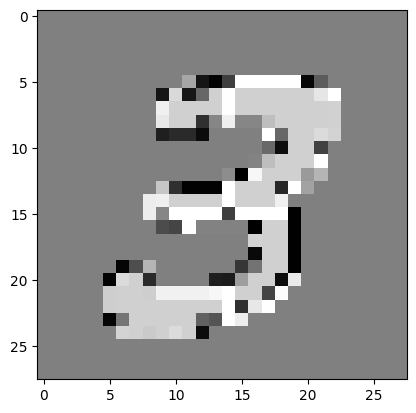
img1 = train_images[7]
print("The image: \n", img1)
print("The label: \n", train_labels[7])  
# display the image
import matplotlib.pyplot as plt
plt.imshow(img1, cmap='gray')

The image: 
 [[  0   0   0   0   0   0   0   0   0   0   0   0   0   0   0   0   0   0
    0   0   0   0   0   0   0   0   0   0]
 [  0   0   0   0   0   0   0   0   0   0   0   0   0   0   0   0   0   0
    0   0   0   0   0   0   0   0   0   0]
 [  0   0   0   0   0   0   0   0   0   0   0   0   0   0   0   0   0   0
    0   0   0   0   0   0   0   0   0   0]
 [  0   0   0   0   0   0   0   0   0   0   0   0   0   0   0   0   0   0
    0   0   0   0   0   0   0   0   0   0]
 [  0   0   0   0   0   0   0   0   0   0   0   0   0   0   0   0   0   0
    0   0   0   0   0   0   0   0   0   0]
 [  0   0   0   0   0   0   0   0   0   0   0  38  43 105 255 253 253 253
  253 253 174   6   0   0   0   0   0   0]
 [  0   0   0   0   0   0   0   0   0  43 139 224 226 252 253 252 252 252
  252 252 252 158  14   0   0   0   0   0]
 [  0   0   0   0   0   0   0   0   0 178 252 252 252 252 253 252 252 252
  252 252 252 252  59   0   0   0   0   0]
 [  0   0   0   0   0   0   0   0   0 109 252 252 230 132 133 132 132 189
  252 252 252 252  59   0   0   0   0   0]
 [  0   0   0   0   0   0   0   0   0   4  29  29  24   0   0   0   0  14
  226 252 252 172   7   0   0   0   0   0]
 [  0   0   0   0   0   0   0   0   0   0   0   0   0   0   0   0   0  85
  243 252 252 144   0   0   0   0   0   0]
 [  0   0   0   0   0   0   0   0   0   0   0   0   0   0   0   0  88 189
  252 252 252  14   0   0   0   0   0   0]
 [  0   0   0   0   0   0   0   0   0   0   0   0   0   0  91 212 247 252
  252 252 204   9   0   0   0   0   0   0]
 [  0   0   0   0   0   0   0   0   0  32 125 193 193 193 253 252 252 252
  238 102  28   0   0   0   0   0   0   0]
 [  0   0   0   0   0   0   0   0  45 222 252 252 252 252 253 252 252 252
  177   0   0   0   0   0   0   0   0   0]
 [  0   0   0   0   0   0   0   0  45 223 253 253 253 253 255 253 253 253
  253  74   0   0   0   0   0   0   0   0]
 [  0   0   0   0   0   0   0   0   0  31 123  52  44  44  44  44 143 252
  252  74   0   0   0   0   0   0   0   0]
 [  0   0   0   0   0   0   0   0   0   0   0   0   0   0   0   0  15 252
  252  74   0   0   0   0   0   0   0   0]
 [  0   0   0   0   0   0   0   0   0   0   0   0   0   0   0   0  86 252
  252  74   0   0   0   0   0   0   0   0]
 [  0   0   0   0   0   0   5  75   9   0   0   0   0   0   0  98 242 252
  252  74   0   0   0   0   0   0   0   0]
 [  0   0   0   0   0  61 183 252  29   0   0   0   0  18  92 239 252 252
  243  65   0   0   0   0   0   0   0   0]
 [  0   0   0   0   0 208 252 252 147 134 134 134 134 203 253 252 252 188
   83   0   0   0   0   0   0   0   0   0]
 [  0   0   0   0   0 208 252 252 252 252 252 252 252 252 253 230 153   8
    0   0   0   0   0   0   0   0   0   0]
 [  0   0   0   0   0  49 157 252 252 252 252 252 217 207 146  45   0   0
    0   0   0   0   0   0   0   0   0   0]
 [  0   0   0   0   0   0   7 103 235 252 172 103  24   0   0   0   0   0
    0   0   0   0   0   0   0   0   0   0]
 [  0   0   0   0   0   0   0   0   0   0   0   0   0   0   0   0   0   0
    0   0   0   0   0   0   0   0   0   0]
 [  0   0   0   0   0   0   0   0   0   0   0   0   0   0   0   0   0   0
    0   0   0   0   0   0   0   0   0   0]
 [  0   0   0   0   0   0   0   0   0   0   0   0   0   0   0   0   0   0
    0   0   0   0   0   0   0   0   0   0]]
The label: 
 3

<matplotlib.image.AxesImage at 0x7f44890d7010>

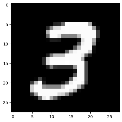
../_images/6af363f365e18d9c9d37e663b01bf405d27edcebdd3d181ae2021239e32a1937.png

img2 = train_images[7] + 100
plt.imshow(img2, cmap='gray')

<matplotlib.image.AxesImage at 0x7f4485765d50>

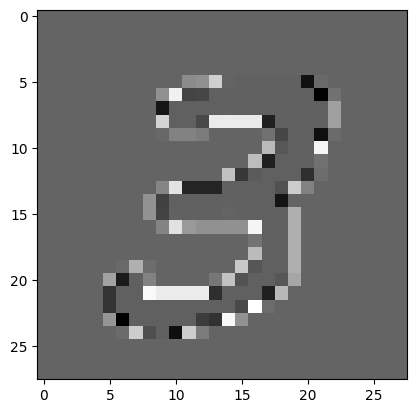
../_images/e5279e117b7f9d7afdae73f62d1d0346c4eba9ae9817ac0f2ab67b0459d4c8e7.png

img2 = np.sin(train_images[7])
plt.imshow(img2, cmap='gray')

<matplotlib.image.AxesImage at 0x7f448353d250>

../_images/b8191a8f12f78aa13c7e199e45ce49d78d5ebb803767536642a38cdd4e7cf27b.png